Tom Adams, Consultant, Sonoscan, Inc.
The echoes are typically gated (by a time window) on a specific internal depth such as the die face, and the transducer pulses VHF or UHF ultrasound at a frequency selected by the user. For a relatively thick package, the operator might select a 10MHz transducer. For a very thin package, he might pick a 300MHz transducer.
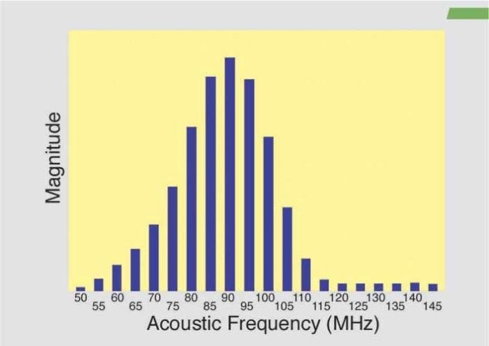
Each transducer actually pulses ultrasound in a spectrum of frequencies around the nominal frequency. Thus, a 230MHz transducer might actually pulse ultrasound from around 160MHz to around 300MHz. The frequency distribution for a typical 100MHz transducer is shown in figure 1. Note that the peak frequency is downshifted from 100MHz to 90MHz due to the differential absorption of ultrasound by this sample and the coupling medium. An AMI-system user making routine planar images is chiefly concerned with the nominal frequency of a transducer, and seldom has reason to think about the range of frequencies involved.
For example, in imaging a flip-chip device, gating of the echo signals is often on the interface between the chip face and the underfill compound, since this is the depth at which anomalies (cracked or sheared solder bumps, voids in the underfill) are likely to occur. As the transducer scans the thousands of XY-locations that make up the area of the flip chip, software routines select the echo signal having the highest amplitude at each XY location to give pixel data for that position. In this process, the frequency content of the echo signal is ignored. Normal planar imaging is therefore known as time-domain imaging, because it depends on the magnitude of the echo signal within a defined time window. The time-domain planar image displays the flip chip as it looks acoustically at the selected depth, and is made from the total echo signals having various frequencies within them.
Recent work at Sonoscan has developed a method that takes advantage of the multiple frequencies available, and that makes it possible to use the company’s C-SAM system to extract previously unavailable data from a sample. For anyone involved in failure analysis, process control or package development, this capability offers a new tool capable of solving difficult packaging-analysis problems. For example, to identify hidden but critical failure mechanisms, harming device reliability.
The newly developed method uses Fast-Fourier Transforms (FFT), to decompose the echo signals from a given XY-location into their frequency spectra. Then unique images can be reconstructed at any frequency or range of frequencies within the spectra. One acoustic image of the selected depth within the sample is made for each frequency. An acoustic scan that produces a single time-domain image might thus produce a large number of these frequency-domain images. If a 230MHz transducer has a frequency spectrum from 160 to 300 MHz, perhaps 30 to 60 useful frequency-domain images might be obtained. An even larger number of images may be produced if the echo signals are decomposed at small frequency intervals (for example: 171MHz, 171.5MHz, etc.) but for too small a frequency difference in the image reconstructions the image contrast changes may not be significant.
These images are generated rapidly, and an observer looking at the whole array of frequency-domain images for a particular package will notice that they differ from each other in contrast. Solder-bump bonds may be a very light gray at 193MHz, for example, and solid black at 194MHz. Other features will show similar changes from one image to the next.
What is not so quickly visible is that the images do not all seem to contain the same information. At first, an observer may notice that details of the traces on the die face are visible at some frequencies but not at other. Closer examination may show that details such as small voids or cracks are visible only at certain frequencies, and that these details may not be visible in the all-frequency time-domain image. These frequency-domain images, in other words, are able to display internal details and features that cannot be seen by any other method.
Figure 2 shows the time-domain image (left) and two frequency-domain images from a flip-chip device. The echo signals were gated on the interface between the die face and the underfill, so that the circular features visible here are not the solder bumps themselves but the bonds between the solder bumps and the die face. The echo signals were decomposed to yield a large number of individual images, including those at the two frequencies (169 and 136MHz) shown here.
The multi-frequency time-domain image shows some of the pattern of metallization on the face of the chip, as well as the solder-bump bonds. Adjacent to two of the solder bumps are white areas that are voids in the cured underfill. No other anomalies are visible.
The 169MHz image has much different contrast, but shows some of the metallization pattern, as well as the two voids, although the voids are shown as outlines at this frequency. In the 136MHz image, the metallization is hardly visible, while the voids stand out sharply. However, something new is seen at 136MHz: three smaller voids (arrows) that are not visible in the time-domain image.
Figure 3 displays the time-domain image (top) and three frequency-domain images at various frequencies showing the three rows of peripheral solder bumps in a flip-chip package. The echo signals were gated at the interface between the solder bumps and the bond pads on the die face.
In the time-domain image, the lighter colored solder-bump bonds are defective There are, however, some visible differences among the defective bonds. The three frequency-domain images give additional information. Near the center of the top row of bumps, for example, is what appears to be a double solder bump (arrow). This anomaly is barely visible in the time-domain image, but stands out clearly in all three frequency-domain images. Therefore, comparison of the images brings out additional details which, with knowledge of the inherently designed structure of the part, can reveal important details about its actual construction and defects.
Summarizing the value of acoustic micro imaging: the advantage lies in the non-destructive method and highly resolved images it provides of internal features, and especially of various types of bonds and disbonds. Frequency-domain acoustic micro imaging makes it possible to image features and details that were previously invisible.
Mit akustischem Micro-Imaging lässt sich zerstörungsfrei das Innere von Halbleitern analysieren. Ein Transducer leitet dazu akustische Signale je nach Anwendung im Bereich von etwa 100 bis über 300 MHz in das Packagematerial ein. Aufgrund der Frequenzdispersion des Transducers (beispielsweise beträgt bei nominal 100 MHz sein Spektrum 55 bis 145 MHz) kommen Signalechos in diesem Bereich zurück, die sehr unterschiedliche Bildinformationen enthalten. Man verwendet diese Informationen von verschiedenen Akustiksignalen, um sehr kritischen, versteckten Fehlermechanismen in IC-Gehäusen auf den Grund zu kommen.
A l’aide de de micro-imagerie acoustique, il est possible d’analyser sans problème l’intérieur de semi-conducteurs. Un transducteur transmet des signaux acoustiques dans la matière du logiciel, selon l’application entre 100 et 300 MHz. Etant donné la dispersion de la fréquence du transducteur (par example son spectre est de 55 à 145 MHz pour 100 MHz nominaux), des échos de signal, qui contiennent des informations images très différentes, reviennent dans ce secteur. Ces informations issues de différents signaux acoustiques sont utilisées pour déceler des erreurs de mécanismes critiques cachées dans les boîtiers IC.
Grazie al Micro-Imaging acustico è possibile analizzare l’interno di semiconduttori, senza temerne alcuna distruzione. A tal fine un trasduttore trasmette segnali acustici a seconda dell’applicazione in un campo compreso all’incirca tra 100 e 300 MHz nel materiale Package. A causa della dispersione di frequenza del trasduttore (ad esempio, in una frequenza nominale di 100 MHz, il suo spettro corrisponde tra 55 e 145 MHz), si verifica una serie di rimbalzi di segnali all’interno di questo campo, comprendenti informazioni d’immagine molto differenti. Queste informazioni provenienti da diversi segnali acustici vengono utilizzate per individuare meccanismi di errore nascosti e molto critici all’interno degli involucri di circuiti integrati.